Factor analysis assume the following[1]: x – mu = LF + epsilon
where L is factor loading, and epsilon is error terms(or uniqueness that’s not explained by common latent factor F).

This is basically saying that x is generated from low dimensional F. F is multiplied by L (so that it can be high dimension), and then finally e is added[2].

In R, we use factanal for factor analysis[4]:

> v1 <- c(1,1,1,1,1,1,1,1,1,1,3,3,3,3,3,4,5,6)
> v2 <- c(1,2,1,1,1,1,2,1,2,1,3,4,3,3,3,4,6,5)
> v3 <- c(3,3,3,3,3,1,1,1,1,1,1,1,1,1,1,5,4,6)
> v4 <- c(3,3,4,3,3,1,1,2,1,1,1,1,2,1,1,5,6,4)
> v5 <- c(1,1,1,1,1,3,3,3,3,3,1,1,1,1,1,6,4,5)
> v6 <- c(1,1,1,2,1,3,3,3,4,3,1,1,1,2,1,6,5,4)
> m1 <- cbind(v1,v2,v3,v4,v5,v6)

> factanal(m1, factors=2, rotation=”none”)
Call:
factanal(x = m1, factors = 2, rotation = “none”)

Uniquenesses:
   v1    v2    v3    v4    v5    v6
0.005 0.114 0.642 0.742 0.005 0.097

Loadings:
   Factor1 Factor2
v1  0.853  -0.518
v2  0.804  -0.490
v3  0.598       
v4  0.508       
v5  0.857   0.510
v6  0.796   0.519

               Factor1 Factor2
SS loadings      3.358   1.038
Proportion Var   0.560   0.173
Cumulative Var   0.560   0.733

Test of the hypothesis that 2 factors are sufficient.
The chi square statistic is 23.14 on 4 degrees of freedom.
The p-value is 0.000119

In this output, uniqueness is variability of variable minus communality (This is actually estimation of epsilon). Communality is diagnonal elements in LLT, i.e., amount of variability explained by common factors, i.e., F.

Below uniqueness, loadings express factor loading matrix. For example, v1 = 0.853 * Factor1 – 0.518 * Factor2. This is estimation of L in the equation.

SS loadings are sum of squares of factor loadings. For example, 3.358 = 0.853^2 + 0.804^2 + 0.598^2 + 0.508^2 + 0.857^2 + 0.796^2. This is amount of variance explained by factors. And in this case, 56%(=0.560) of variance is explained by Factor1.

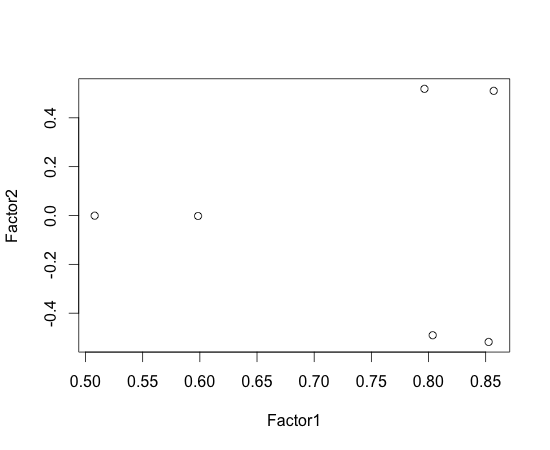
Finally, there’s chi squre fit test to see if 2 factors explain m1. Here, as p-value 0.000119 < 0.05, it does not explain the data very well (as alternative hypothesis is accepted while our H0 is “2 factors are sufficient”). If we plot factor loadings, we can group variables easily based on factor affecting them, e.g.: [code lang="R"] > f = factanal(m1, factors=2, rotation=”none”) > plot(f$loadings) [/code]

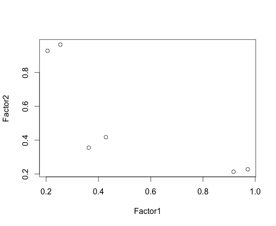
In the above, we see there are two groups whose Factor1 is large while their Factor2 is different. This makes grouping difficult. To solve this problem, we can use factor rotation. In the below, I used varimax (this is default of factanal; I’ve specified rotation=”none” in the above on purpose).

> varimax(f$loadings)$loadings

Loadings:
   Factor1 Factor2
v1 0.971   0.228 
v2 0.917   0.213 
v3 0.429   0.418 
v4 0.363   0.355 
v5 0.254   0.965 
v6 0.205   0.928 

               Factor1 Factor2
SS loadings      2.206   2.190
Proportion Var   0.368   0.365
Cumulative Var   0.368   0.733

> plot(varimax(f$loadings)$loadings)

Or, we could have used factanal without specifying rotation to use varimax:

> factanal(m1, factors=2)

Varimax is orthogonal rotation. In other words, it rotates Factor1 and Factor2 axes while keeping their angle right(90 degree). However, there are other rotation like covarimin, quartimin, oblimin(this is popular one) which does not keep the right angle.

References:
1) Wikipedia. http://en.wikipedia.org/wiki/Factor_analysis
2) Machine learning lecture 13 by Andrew Ng. http://www.youtube.com/watch?v=LBtuYU-HfUg&feature=player_detailpage#t=1885s
3) 이용구, 김성수, 김현중, “다변량 분석 입문”, Knou Press.
4) help(factanal) in R.