Let’s assume two class(A and B) classification. Also assume that a classification algorithm predicts that the given data is class A with probability 0.8. To predict if it’s class A or B, we need a threshold parameter (i.e., cutoff).
If 0.8 is higher then the threshold , we’ll predict that the data is class A. Otherwise, we’ll predict the data is from class B.
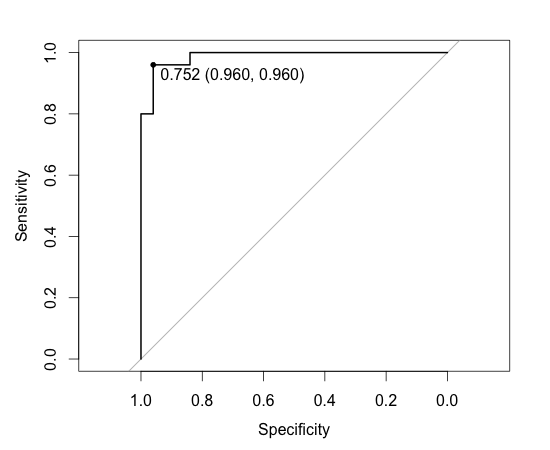
ROC graph can be used for this purpose. If we think sensitivity and specificity is equally important, we just need to set the threshold to the top left corner of the graph. Below is an example of this in R.
> library(caret)
> library(pROC)
> data(iris)

> # Make this two class classification.
> iris <- iris[iris$Species == "virginica" | iris$Species == "versicolor", ]
> iris$Species <- factor(iris$Species)  # setosa should be removed from factor
> levels(iris$Species)
[1] "versicolor" "virginica"

> # Get train and test datasets.
> # I'm making train set very small intentionally so that we get some wrong classification
> # results. This will give ROC graph some curves.
> samples <- sample(NROW(iris), NROW(iris) * .5)
> data.train <- iris[samples, ]
> data.test <- iris[-samples, ]

> # Random forest
> forest.model <- train(Species ~., data.train)
> forest.model
50 samples
 4 predictors
 2 classes: 'versicolor', 'virginica'

No pre-processing
Resampling: Bootstrap (25 reps)

Summary of sample sizes: 50, 50, 50, 50, 50, 50, ...

Resampling results across tuning parameters:

  mtry  Accuracy  Kappa  Accuracy SD  Kappa SD
  2     0.928     0.855  0.0532       0.105
  3     0.924     0.849  0.0569       0.113
  4     0.917     0.834  0.0625       0.123

Accuracy was used to select the optimal model using  the largest value.
The final value used for the model was mtry = 2.

> # Prediction.
> result.predicted.prob <- predict(forest.model, data.test, type="prob")

> # Draw ROC curve.
> result.roc <- roc(data.test$Species, result.predicted.prob$versicolor)
> plot(result.roc, print.thres="best", print.thres.best.method="closest.topleft")

Call:
roc.default(response = data.test$Species, predictor = result.predicted.prob$versicolor)

Data: result.predicted.prob$versicolor in 25 controls (data.test$Species versicolor) > 25 cases (data.test$Species virginica).
Area under the curve: 0.9872

> # Get some more values.
> result.coords <- coords(
+   result.roc, "best", best.method="closest.topleft", ret=c("threshold", "accuracy"))

> print(result.coords)
threshold  accuracy
    0.752     0.960

> # Make prediction using the best top-left cutoff.
> result.predicted.label <- factor(
    ifelse(result.predicted.prob[,1] > result.coords[1], "versicolor", "virginica"))

> xtabs(~  result.predicted.label + data.test$Species)
                      data.test$Species
result.predicted.label versicolor virginica
            versicolor         24         1
            virginica           1        24
The accuracy was 0.960 when the threshold was set to 0.752 which is the same with (24+24)/(24+1+1+24) in the cross tabulation. Note that this accuracy is different form the accuracy shown by ‘forest.model’. forest.model’s accuracy is estimated by cross validation of data.train, hence it’s smaller. Below is ROC curve.

Instead of using top left corner, we may pick the threshold that maximize ‘sensitivity + specificity’ or some weighted version of it. See help(coords) for this purpose.