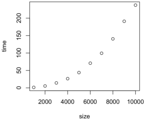
Training time becomes an issue, esp., if someone is using complicated model like svm with huge data. When that happens, it’s critical to estimate when the training will end. I’ve written a simple R code to do that efficiently (in terms of time but not in terms of accuracy).

> # Load your data into 'train'.
> 
> # I'll use svm.
> library(e1071)
> # Will use parallelization.
> library(doMC)
> 
> # Set the number of workers to the number of cores.
> registerDoMC()
> 
> # Time with svm for data size 1000, 2000, 3000, ..., 10000.
> # And estimate the time in parallel!
> results <- foreach(i=seq(1000, 10000, 1000)) %dopar% {
+   print(i)
+   start <- proc.time()
+   sub_train <- svm(label ~., data=train[1:i,], kernel='linear')
+   end <- proc.time()
+   return(list(size=i, time=(end - start)[3]))
+ }
[1] 1000
[1] 2000
[1] 3000
[1] 4000
[1] 5000
[1] 6000
[1] 7000
[1] 8000
[1] 9000
[1] 10000
> results
[[1]]
[[1]]$size
[1] 1000

[[1]]$time
elapsed 
   1.33 


[[2]]
[[2]]$size
[1] 2000

[[2]]$time
elapsed 
  5.845 

... omitted ...

> # Convert the list into data frame.
> time_taken <- as.data.frame(matrix(unlist(results), ncol=2, byrow=T))
> colnames(time_taken) <- c("size", "time")
> time_taken
    size    time
1   1000   1.330
2   2000   5.845
3   3000  13.934
4   4000  26.413
5   5000  45.508
6   6000  67.102
7   7000  96.151
8   8000 135.744
9   9000 183.990
10 10000 229.421
> # Let's see if time = a * size + b * size^2 + c * size^3 + d * size^4 + error.
> m <- lm(time ~ poly(size, 4), data=time_taken)
> summary(m)

Call:
lm(formula = time ~ poly(size, 4), data = time_taken)

Residuals:
      1       2       3       4       5       6       7       8       9      10 
 0.5405 -0.9368 -0.5183  0.3327  2.1665 -0.2056 -2.2956 -0.8783  2.8949 -1.1001 

Coefficients:
               Estimate Std. Error t value Pr(>|t|)    
(Intercept)     80.5438     0.6621 121.654 7.12e-10 ***
poly(size, 4)1 227.8825     2.0937 108.844 1.24e-09 ***
poly(size, 4)2  69.3148     2.0937  33.107 4.73e-07 ***
poly(size, 4)3   4.3338     2.0937   2.070   0.0932 .  
poly(size, 4)4  -3.2294     2.0937  -1.542   0.1836    
---
Signif. codes:  0 ‘***’ 0.001 ‘**’ 0.01 ‘*’ 0.05 ‘.’ 0.1 ‘ ’ 1 

Residual standard error: 2.094 on 5 degrees of freedom
Multiple R-squared: 0.9996,	Adjusted R-squared: 0.9993 
F-statistic:  3237 on 4 and 5 DF,  p-value: 1.024e-08 

> # Find the highest order whose p-value is bigger than 0.05. 
> # In this case, size^3 has p-value 0.0932 > 0.05. Thus, ignore terms
> # with order greater than or equal to 3. So, the model will be 
> # time = a * size + b * size^2 + error.
>
> # Note that, even if p-value of size^1 is larger than 0.05, we won't 
> # ignore size^1 term as size^2 is significant.
>
> # Predict the total time to train all data.
> predict(lm(time ~ poly(size, 2), data=time_taken), data.frame(size=nrow(train)))
       1 
91304.46 
> # It will take 1.06 day.
> 91304.46 / 60 / 60 / 24
[1] 1.056765

Here’s the graph: