This is follow up on the previous posting ANOVA IN R.
In R, whether we have different number of repeated experiments does not matter when executing aov(). Given four different systems a1, a2, a3 and a4 and measurements, I’ll describe how we check if their means are different, how we get confidence interval at each level and how we get pairs with statistically significant different means.
First, enter data as data frame, then convert it using melt().
> d = list(a1=c(38, 41, 37, 36, 42),
+          a2=c(43, 47, 41, 54, 55, 48),
+          a3=c(30, 35, 22, 37, 38, 27),
+          a4=c(46, 41, 43, 45, 48, 47))
> d
$a1
[1] 38 41 37 36 42

$a2
[1] 43 47 41 54 55 48

$a3
[1] 30 35 22 37 38 27

$a4
[1] 46 41 43 45 48 47

> library(reshape)
> md = melt(d)
> md
   value L1
1     38 a1
2     41 a1
3     37 a1
4     36 a1
5     42 a1
6     43 a2
7     47 a2
8     41 a2
9     54 a2
10    55 a2
11    48 a2
12    30 a3
13    35 a3
14    22 a3
15    37 a3
16    38 a3
17    27 a3
18    46 a4
19    41 a4
20    43 a4
21    45 a4
22    48 a4
23    47 a4

> # Don't forget!
> md$L1 <- factor(md$L1)
Alternatively, one can use stack() for this conversion.
> stack(d)
   values ind
1      38  a1
2      41  a1
3      37  a1
4      36  a1
5      42  a1
6      43  a2
7      47  a2
8      41  a2
9      54  a2
10     55  a2
11     48  a2
12     30  a3
13     35  a3
14     22  a3
15     37  a3
16     38  a3
17     27  a3
18     46  a4
19     41  a4
20     43  a4
21     45  a4
22     48  a4
23     47  a4
> f = stack(d)
> class(f)
[1] "data.frame"
> str(f)
'data.frame':	23 obs. of  2 variables:
 $ values: num  38 41 37 36 42 43 47 41 54 55 ...
 $ ind   : Factor w/ 4 levels "a1","a2","a3",..: 1 1 1 1 1 2 2 2 2 2 ...
Let’s get means in each group in interesting ways.
> library(reshape)
> ddply(md, .(L1), summarise, mean_value=mean(value))
  L1 mean_value
1 a1       38.8
2 a2       48.0
3 a3       31.5
4 a4       45.0

> with(md, by(value, L1, mean))
L1: a1
[1] 38.8
------------------------------------------------------------
L1: a2
[1] 48
------------------------------------------------------------
L1: a3
[1] 31.5
------------------------------------------------------------
L1: a4
[1] 45

> with(md, tapply(value, L1, mean))
  a1   a2   a3   a4
38.8 48.0 31.5 45.0
All of the above work. So it’s your choice how you get the means.
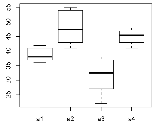
Now, draw a boxplot to check differences visually.
> with(md, boxplot(value ~ L1))

Run anova.
> model = aov(value ~ L1, md)
> anova(model)
Analysis of Variance Table

Response: value
          Df Sum Sq Mean Sq F value    Pr(>F)
L1         3 955.53  318.51  14.467 3.816e-05 ***
Residuals 19 418.30   22.02
---
Signif. codes:  0 ‘***’ 0.001 ‘**’ 0.01 ‘*’ 0.05 ‘.’ 0.1 ‘ ’ 1
There is at least one level whose mean is different from others.
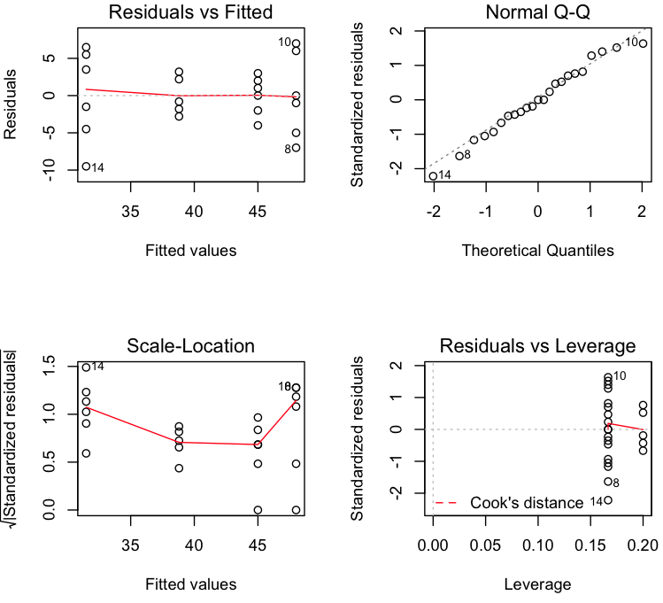
Diagnose the model.
> par(mfrow=c(2,2))
> plot(model)

Residual vs Fitted looks fine as residuals looks randomly distributed. Normal Q-Q plot tells us residuals are almost gaussian.
As anova is basically linear regression, we get confidence interval by:
> confint(model)
                  2.5 %    97.5 %
(Intercept)  34.4080605 43.191940
L1a2          3.2532858 15.146714
L1a3        -13.2467142 -1.353286
L1a4          0.2532858 12.146714
So, a1’s conf. interval is [34.41, 43.19], and so on.
To find out pairs of levels with statistically different means, we use TukeyHSD.
> hsd = TukeyHSD(model, "L1", ordered=TRUE)
> hsd
  Tukey multiple comparisons of means
    95% family-wise confidence level
    factor levels have been ordered

Fit: aov(formula = value ~ L1, data = md)

$L1
      diff        lwr      upr     p adj
a1-a3  7.3 -0.6890361 15.28904 0.0806685
a4-a3 13.5  5.8827530 21.11725 0.0004414
a2-a3 16.5  8.8827530 24.11725 0.0000408
a4-a1  6.2 -1.7890361 14.18904 0.1641134
a2-a1  9.2  1.2109639 17.18904 0.0206317
a2-a4  3.0 -4.6172470 10.61725 0.6894454

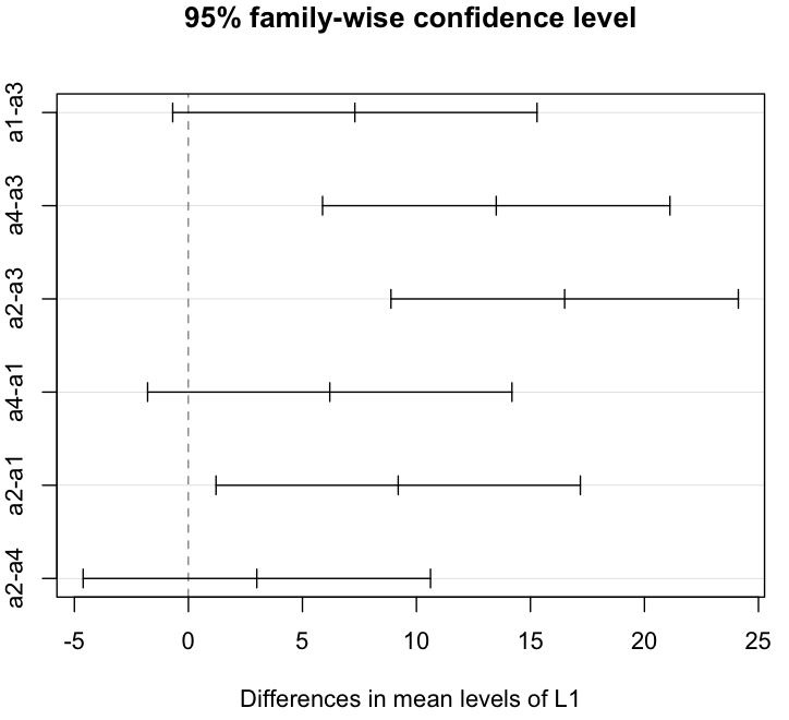
> plot(hsd)

It’s much easier to figure out pairs with plot. As one can see, a4-a3, a2-a3, a2-a1 are pairs with meaningful mean differences.
Refernces)
1. 김재희, R을이용한통계프로그래밍기초, 자유아카데미
2. 임용빈외, 실험계획과응용, KNOUPRESS