Let’s use caret to find out the better # of hidden nodes.
library(neuralnet)
library(caret)
In the below, I needed many data so that default sampling method, i.e., k-fold CV, can have enough data in it. (i.e., if k=5 or 10, how can we run k-fold using just 4 data rows?) We may choose to instantiate trainControl, but I didn’t.
> data = data.frame(x1=rep(c(0,0,1,1),100), x2=rep(c(0,1,0,1),100), y=rep(c(0,1,1,0),100))
Repeat 5 times for each random initial weights, and test “which is better between one hidden node and two?”.
> fit <- train(data[,-3], data[,3], method="neuralnet", rep=5, tuneGrid=expand.grid(.layer1=c(1,2), .layer2=0, .layer3=0))
> fit
0 samples
  2 predictors

No pre-processing
Resampling: Bootstrap (25 reps)

Summary of sample sizes: 400, 400, 400, 400, 400, 400, ...

Resampling results across tuning parameters:

  layer1  RMSE   Rsquared  RMSE SD  Rsquared SD
  1       0.417  0.309     0.0104   0.0338
  2       0.179  0.731     0.191    0.292

Tuning parameter 'layer2' was held constant at a value of 0
Tuning parameter 'layer3' was held constant at
 a value of 0
RMSE was used to select the optimal model using  the smallest value.
The final values used for the model were layer1 = 2, layer2 = 0 and layer3 = 0.
It said layer1 (first hidden layer) performs better when there are two nodes. Check out the best model.
> print(fit$finalModel)
Call: neuralnet(formula = form, data = data, hidden = nodes, rep = 5)

5 repetitions were calculated.

              Error Reached Threshold Steps
3 0.000001375257340    0.008889472935   111
1 0.000001847984922    0.005850881101   177
5 0.000002766922207    0.008386811191   140
4 0.000006304931444    0.009817355091   152
2 0.000012174188912    0.009405383907   125
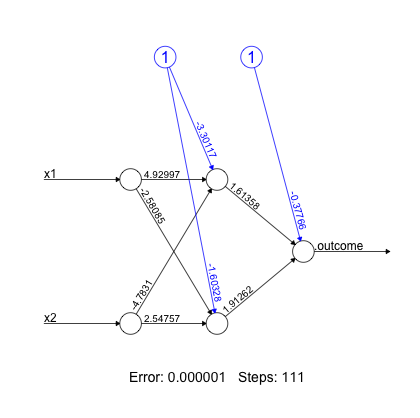
This had 5 repetitions in it. Among then, third (error=0.0000013752…) is the best. Plot it.
> plot(fit$finalModel, rep="best")
Check out the prediction. (Note: It’s ‘prediction’ and not ‘predict’ in neuralnet package).
> prediction(fit$finalModel)
Data Error:	0;
$rep1
  x1 x2        .outcome
1  0  0 0.0001132194082
2  1  0 0.9999376943012
3  0  1 0.9999032236447
4  1  1 0.0001043714568

$rep2
  x1 x2         .outcome
1  0  0  0.0004353878876
2  1  0  0.9999684529385
3  0  1  0.9998948154582
4  1  1 -0.0002046024453

$rep3
  x1 x2          .outcome
1  0  0 0.000083067082225
2  1  0 1.000001256836959
3  0  1 0.999856492690309
4  1  1 0.000003013149072

$rep4
  x1 x2         .outcome
1  0  0 0.00017557506929
2  1  0 0.99971323908940
3  0  1 0.99993048205920
4  1  1 0.00009059503288

$rep5
  x1 x2          .outcome
1  0  0 0.000001700996794
2  1  0 0.999840441840330
3  0  1 0.999996792653854
4  1  1 0.000172819146397

$data
  x1 x2 .outcome
1  0  0        0
2  1  0        1
3  0  1        1
4  1  1        0
Among them, $rep3 is the best. There’s no way to pick $rep3 only in prediction function, but we can do so with compute. With compute, one can check the neuralnet with some input that didn’t exist in the training data, as well. Sadly, rep=”best” does not work with compute, so we should pick one by specifying rep #.
> compute(fit$finalModel, data.frame(x1=0, x2=1), rep = 3)
$neurons
$neurons[[1]]
     1 x1 x2
[1,] 1  0  1

$neurons[[2]]
     [,1]            [,2]         [,3]
[1,]    1 0.0003082565774 0.7199652986


$net.result
             [,1]
[1,] 0.9998564927
See that $net.result is almost equals to 1.
In this example, we did’t need any scaling as the input lies within [0, 1]. However, in general, we need to use preProcess() to scale input. This is due to Komogorov’s proof that any continuous function lies within hypercube [0, 1] can be approximated by three layer neural net like model assuming the proper number of hidden layer nodes. See pateern classification by Duda for details.
For neuralnet, see:
1) http://journal.r-project.org/archive/2010-1/RJournal_2010-1_Guenther+Fritsch.pdf
2) http://cran.r-project.org/web/packages/neuralnet/
