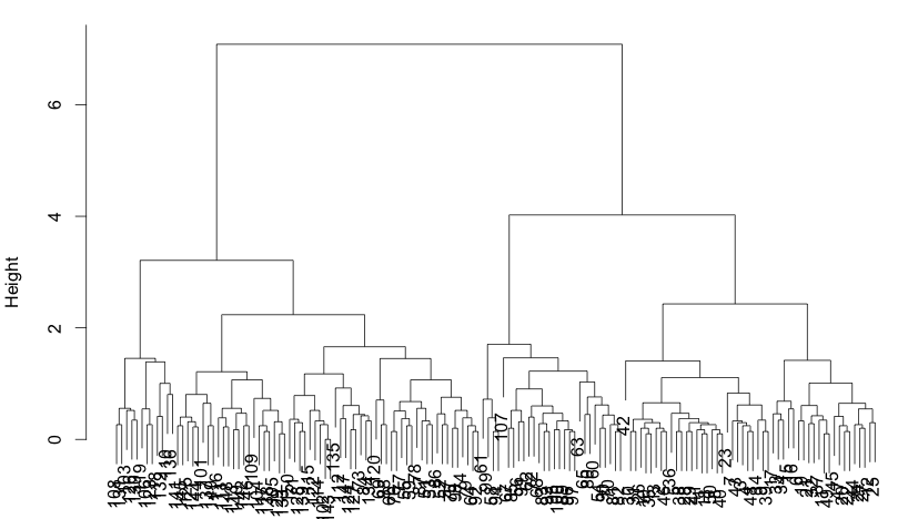
First, remove species:

> i = as.matrix(iris[,-5])
> i[1:5,]
     Sepal.Length Sepal.Width Petal.Length Petal.Width
[1,] “5.1″        ”3.5″       “1.4″        ”0.2″     
[2,] “4.9″        ”3.0″       “1.4″        ”0.2″     
[3,] “4.7″        ”3.2″       “1.3″        ”0.2″     
[4,] “4.6″        ”3.1″       “1.5″        ”0.2″     
[5,] “5.0″        ”3.6″       “1.4″        ”0.2″    

Draw hierarchical clustering:

> hc = hclust(dist(i))
> plclust(hc)

It’s very tempting to pick three clusters as we already know that there are three species. So, cut cluster at three:

> kls = cutree(hc, 3)
> kls
  [1] 1 1 1 1 1 1 1 1 1 1 1 1 1 1 1 1 1 1 1 1 1 1 1 1 1 1 1 1 1 1 1
 [32] 1 1 1 1 1 1 1 1 1 1 1 1 1 1 1 1 1 1 1 2 2 2 3 2 3 2 3 2 3 3 3
 [63] 3 2 3 2 3 3 2 3 2 3 2 2 2 2 2 2 2 3 3 3 3 2 3 2 2 2 3 3 3 2 3
 [94] 3 3 3 3 2 3 3 2 2 2 2 2 2 3 2 2 2 2 2 2 2 2 2 2 2 2 2 2 2 2 2
[125] 2 2 2 2 2 2 2 2 2 2 2 2 2 2 2 2 2 2 2 2 2 2 2 2 2 2

Now we got three clusters for the iris data. We can check it’s accuracy using table:

> table(iris$Species, kls)
            kls
              1  2  3
  setosa     50  0  0
  versicolor  0 23 27
  virginica   0 49  1

It’s easy to see that versicolor is often confused with virginica in this approach.
Instead of hierarchical clustering, we can try divisive clustering. Unlike hierarchical one, it considers global distribution, so it performs better sometimes[1]. Also, it’s faster as it does not need to compute distance for every pairs[2].

> da = diana(i)
> table(iris$Species, cutree(da, 3))
            
              1  2  3
  setosa     50  0  0
  versicolor  3 46  1
  virginica   0 14 36

Finally, here’s kmeans:

> km = kmeans(i, 3)
> table(km$cluster, iris$Species)
   
    setosa versicolor virginica
  1     17          4         0
  2     33          0         0
  3      0         46        50

References)
1. Divisive Clustering. http://nlp.stanford.edu/IR-book/html/htmledition/divisive-clustering-1.html
2. 구자용, 박헌진, 최대우, 김성수, “데이터 마이닝”, Knou Press.