Principal component analysis (PCA) is a mathematical procedure that uses an orthogonal transformation to convert a set of observations of possibly correlated variables into a set of values of uncorrelated variables called principal components[1]. PCA tries to reduce dimension while maintaining axis which has the largest variance. And the problem boils down to getting principal eigen vectors of X[2].
PCA model[3] is PC=Xp where PC is principal component score matrix. p is the matrix of eigenvector of correlation of X. Here, we assume X is scaled (z score). If so, (PC)’PC=(Xp)’(Xp) = p’X’Xp. Because we’re seeking for PC whose scores are independent each other, (PC)’(PC) is diagonal matrix whose main diagonal contains squares of principal scores. Also, X’X is sum of squares and cross product of X.
If we divide both side by n, then W = p’Ap, and A=pWp’ where A is correlation matrix of X, p is eigenvectors of A and W is eigenvalue matrix.
For example, given the following x[I’m solving the exercise problems using R at p77, Exercies 4.7-4.10 of Reference #3]:
> x
     [,1] [,2]
[1,]  120  140
[2,]   90  110
[3,]  100   90
[4,]  110  120
[5,]  115  130
Scale it first (sqrt(5/4) is for dividing by 5 when computing standard deviation and not by 4):
> scale(x) * sqrt(5/4)
           [,1]       [,2]
[1,]  1.2070197  1.2787240
[2,] -1.5784104 -0.4649906
[3,] -0.6499337 -1.6274669
[4,]  0.2785430  0.1162476
[5,]  0.7427814  0.6974858
attr(,”scaled:center”)
[1] 107 118
attr(,”scaled:scale”)
[1] 12.04159 19.23538
And we get correlation matrix:
> sx = scale(x) * sqrt(5/4)
> t(sx) %*% sx / 5
          [,1]      [,2]
[1,] 1.0000000 0.7771192
[2,] 0.7771192 1.0000000
We get eigen vector / values like:
> a = t(sx) %*% sx / 5
> eigen(a)
$values
[1] 1.7771192 0.2228808

$vectors
          [,1]       [,2]
[1,] 0.7071068 -0.7071068
[2,] 0.7071068  0.7071068
Correlation can be reconstructed like:
> ev = diag(eigen(a)$values)
> et = eigen(a)$vectors
> et %*% ev %*% t(et)
          [,1]      [,2]
[1,] 1.0000000 0.7771192
[2,] 0.7771192 1.0000000
In other words, we’ve decomposed correlation matrix like the above using eigen vectors and values, and this is called spectral decomposition.
Finally, we get PC = Xp:
> sx %*% et
           [,1]        [,2]
[1,]  1.7576862  0.05070262
[2,] -1.4449027  0.78730670
[3,] -1.6103654 -0.69122040
[4,]  0.2791591 -0.11476016
[5,]  1.0184227 -0.03202877
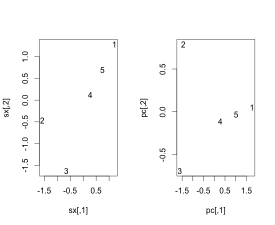
If we draw scaled x and pc:
> par(mfrow=c(1,2))
> plot(sx, type=”n”)
> text(x=sx[,1], y = sx[,2], label=c(1, 2, 3, 4, 5), ex=1)
> pc = sx %*% et
> plot(pc, type=”n”)
> text(x=pc[,1], y = pc[,2], label=c(1, 2, 3, 4, 5), ex=1)
We surely can use princomp:
> princomp(x, cor=T)
Call:
princomp(x = x, cor = T)

Standard deviations:
   Comp.1    Comp.2
1.3330863 0.4721025

 2  variables and  5 observations.
Here, ‘Standard deviations’ are standard deviation of pc. Therefore, 1.3330863 ** 2 = 1.777119 which is the same with eigenvalue of the first column of pc matrix. The same is true for 0.4721025 ** 2. To get scores:
> princomp(x, cor=T)$scores
         Comp.1      Comp.2
[1,] -1.7576862 -0.05070262
[2,]  1.4449027 -0.78730670
[3,]  1.6103654  0.69122040
[4,] -0.2791591  0.11476016
[5,] -1.0184227  0.03202877
To get eigen vectors:
> princomp(x, cor=T)$loadings

Loadings:
     Comp.1 Comp.2
[1,] -0.707  0.707
[2,] -0.707 -0.707

               Comp.1 Comp.2
SS loadings       1.0    1.0
Proportion Var    0.5    0.5
Cumulative Var    0.5    1.0
See that ‘Loadings’ in the above is the same as eigen(a)$vectors.
To measure how much information each of Comp.1 and Comp.2 delivers, we can use eigenvalues.
> eigen(a)$values
[1] 1.7771192 0.2228808
Therefore, Comp.1′s variance corresponds to 1.777/(1.7771192+0.2228808) = 88.9%.
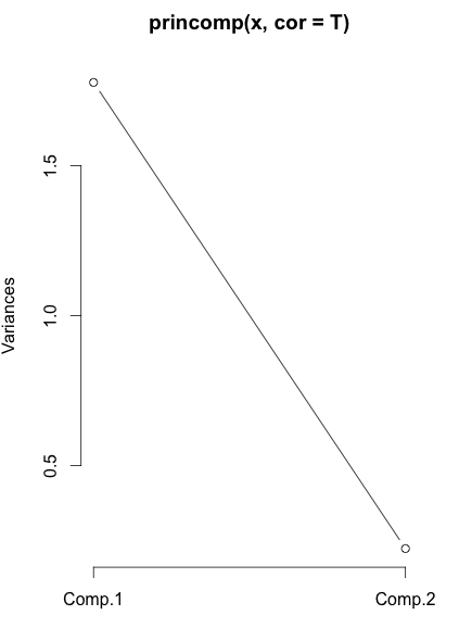
We can use eigen(a)$values to decide the number of dimension of pc. Also, we can use scree plot[3, 4]:
> plot(princomp(x, cor=T), type=”l”)
In this plot, y axis is variance of principal components, i.e., eigen value.
There are other interesting things like factor pattern matrix which measures correlation between X and PC, but it does not look like R has a function to easily do that (though we can compute it by ourselves).
References)
1. Wikipedia entry on PCA. http://en.wikipedia.org/wiki/Principal_component_analysis
2. Machine learning lecture note by Andrew Ng. http://www.stanford.edu/class/cs229/notes/cs229-notes10.pdf
3. 박광배, “다변량분석”, 학지사.
4. 정강모, 김명근, “R기반 다변량 분석, 교우사.

