Let’s build artificial data:
> x = 1:100
> y = 3*x + rnorm(100, 0, 0.1)
Now, y has 3*x + error (which follows independent normal distribution.)
> y
  [1]   3.084463   5.921660   9.043298  11.863854  14.975701  17.980051  20.812897  23.950546  27.013619  29.879748  33.029797
 [12]  35.933785  39.032856  42.021709  45.150473  47.988470  51.005696  53.921992  56.956936  60.154561  62.870397  66.056555
 [23]  68.818562  71.878614  75.037485  77.971538  81.212420  84.075885  86.924858  89.879004  92.987709  96.250259  98.866730
 [34] 101.816094 104.976485 108.138008 111.180993 114.016497 117.019846 119.892135 123.005147 125.958263 129.165459 131.892357
 [45] 134.985222 137.992608 141.158806 144.089719 146.924594 149.944683 153.130148 156.113614 158.992470 162.068371 165.093236
 [56] 168.134131 171.038950 174.138382 176.801168 180.132722 183.137894 185.884679 188.922193 192.098572 195.171722 198.037255
 [67] 201.071104 204.023956 206.970078 209.960827 212.839931 215.842587 218.939796 221.790648 225.065676 228.100543 231.090998
 [78] 233.996619 236.942362 239.952409 242.805987 246.144036 248.835554 251.792460 255.217650 257.822964 260.989347 264.009189
 [89] 267.065940 270.070240 272.876032 275.924888 279.106800 282.153525 284.942045 288.031658 290.881470 293.930968 296.895243
[100] 299.968869
Build a model:
> m = lm(y ~ x)
> m

Call:
lm(formula = y ~ x)

Coefficients:
(Intercept)            x
 -1.168e-05    3.000e+00
This shows that yhat = 3.0 * x – 1.168e-05. Let’s check the goodness of this model:
> summary(m)

Call:
lm(formula = y ~ x)

Residuals:
      Min        1Q    Median        3Q       Max
-0.204330 -0.074342 -0.004509  0.079480  0.252437

Coefficients:
              Estimate Std. Error  t value Pr(>|t|)
(Intercept) -1.168e-05  2.239e-02   -0.001        1
x            3.000e+00  3.849e-04 7793.923   —
Signif. codes:  0 ‘***’ 0.001 ‘**’ 0.01 ‘*’ 0.05 ‘.’ 0.1 ‘ ’ 1

Residual standard error: 0.1111 on 98 degrees of freedom
Multiple R-squared:     1,	Adjusted R-squared:     1
F-statistic: 6.075e+07 on 1 and 98 DF,  p-value: < 2.2e-16
Adjusted R-squared says that 100% of variation is explained by this linear regression, and we can see that t value of x has p < 0.05 meaning that x is statistically meaningful in this model. It’s easy to draw some diagrams:
> par(mfrow=c(2,2))
> plot(m)

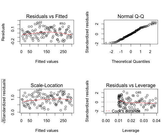
Residual VS Fitted looks fine (though it would have been much nicer if the line were totally flat). Normal Q-Q plot shows us that residual follows a normal distribution.
Let’s make an intentional mistake. In the following we will try to model y = ax + bz + c while y is actually 3x + error:
> z = runif(100, 0, 50)
> m2 = lm (y ~ x + z)
> m2

Call:
lm(formula = y ~ x + z)

Coefficients:
(Intercept)            x            z
  0.0052540    2.9999384   -0.0002374

> summary(m2)

Call:
lm(formula = y ~ x + z)

Residuals:
      Min        1Q    Median        3Q       Max
-0.199865 -0.075759 -0.007949  0.077534  0.256803

Coefficients:
              Estimate Std. Error  t value Pr(>|t|)
(Intercept)  0.0052540  0.0284124    0.185    0.854
x            2.9999384  0.0003872 7747.345   z           -0.0002374  0.0007824   -0.303    0.762
—
Signif. codes:  0 ‘***’ 0.001 ‘**’ 0.01 ‘*’ 0.05 ‘.’ 0.1 ‘ ’ 1

Residual standard error: 0.1116 on 97 degrees of freedom
Multiple R-squared:     1,	Adjusted R-squared:     1
F-statistic: 3.009e+07 on 2 and 97 DF,  p-value: < 2.2e-16
As one can see, z’s p value is 0.762 which is larger than 0.05 meaning that the value is not useful in modeling. Let’s compare m and m2 using ANOVA:
> anova(m, m2)
Analysis of Variance Table

Model 1: y ~ x
Model 2: y ~ x + z
  Res.Df    RSS Df Sum of Sq     F Pr(>F)
1     98 1.2098
2     97 1.2087  1 0.0011466 0.092 0.7623
This shows that the model 2 is not too different from model 1 (as p value 0.7623 is larger than 0.05, they’re not statistically different model.) Therefore, it’s fine to think that z is meaningless. (Recall that p value of z shows that z is not meaningful.)
We may find y ~ x starting from y ~ x + z automatically:
> step(m2, scope=list(lower=y ~ 1, direction=”backward”))
Start:  AIC=-435.57
y ~ x + z

       Df Sum of Sq    RSS     AIC
- z     1         0      1 -437.47
                   1 -435.57
- x     1    747884 747885  895.98

Step:  AIC=-437.47
y ~ x

       Df Sum of Sq    RSS     AIC
                   1 -437.47
- x     1    749891 749892  894.25

Call:
lm(formula = y ~ x)

Coefficients:
(Intercept)            x
 -1.168e-05    3.000e+00
Final model from step was y ~ x. When we removed z, AIC became -437.47 while AIC of y ~ x + z was -435.57 (smaller AIC is better).
Let’s perform boxcox transformation. For that, let’s change x to sqrt(x):
> x = 1:100
> y = 3 * x + rnorm(100, 0, 0.1)
> x = sqrt(x)
> m3 = lm(y ~ x)
> summary(m3)

Call:
lm(formula = y ~ x)

Residuals:
    Min      1Q  Median      3Q     Max
-17.535 -14.181  -4.509  11.042  60.449

Coefficients:
            Estimate Std. Error t value Pr(>|t|)
(Intercept) -93.8145     5.1147  -18.34   x            36.5330     0.7197   50.76   —
Signif. codes:  0 ‘***’ 0.001 ‘**’ 0.01 ‘*’ 0.05 ‘.’ 0.1 ‘ ’ 1

Residual standard error: 16.75 on 98 degrees of freedom
Multiple R-squared: 0.9634,	Adjusted R-squared: 0.963
F-statistic:  2576 on 1 and 98 DF,  p-value: < 2.2e-16
This model looks good, but boxcox transformation may make it better:
> library(MASS)
> boxcox(m3)
> bc = boxcox(m3)
> bc$x[which.max(bc$y)]
[1] 0.5050505
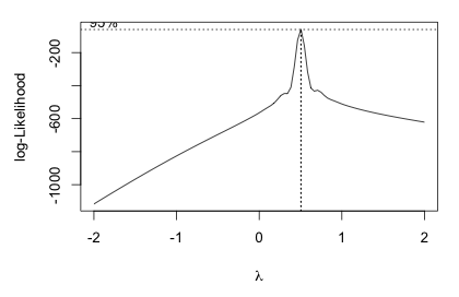
bc$x and bc$y are points in the above plot. Thus, we can see that lambda = 0.5050505 has max. likelihood. To apply that:
> m4 = lm(I(y^0.5050505) ~ x)
> summary(m4)

Call:
lm(formula = I(y^0.5050505) ~ x)

Residuals:
      Min        1Q    Median        3Q       Max
-0.020409 -0.008784 -0.001066  0.006676  0.091507

Coefficients:
              Estimate Std. Error t value Pr(>|t|)
(Intercept) -0.0916328  0.0044541  -20.57   x            1.7903556  0.0006268 2856.43   —
Signif. codes:  0 ‘***’ 0.001 ‘**’ 0.01 ‘*’ 0.05 ‘.’ 0.1 ‘ ’ 1

Residual standard error: 0.01458 on 98 degrees of freedom
Multiple R-squared:     1,	Adjusted R-squared:     1
F-statistic: 8.159e+06 on 1 and 98 DF,  p-value: < 2.2e-16
Now we have much better Adjusted R-square. Or we may do forward-backward selection:
> m5 = lm(y ~ 1)
> step(m5, list(lower=y~1, upper=y~x+z), direction=”both”)
Start:  AIC=894.27
y ~ 1

       Df Sum of Sq    RSS    AIC
+ x     1    722550  27484 565.62
              750034 894.27
+ z     1      2015 748019 896.00

Step:  AIC=565.62
y ~ x

       Df Sum of Sq    RSS    AIC
               27484 565.62
+ z     1        45  27439 567.46
- x     1    722550 750034 894.27

Call:
lm(formula = y ~ x)

Coefficients:
(Intercept)            x
     -93.81        36.53
But this is not a silver bullet; it’s better to find better feature in the first place.
References)
1. R Cookbook by Paul Teetor. Copyright 2011 Paul Teetor, 978-0-596-80915-7.
2. 구자용, 박현진, 최대우, 김성수, 데이터마이닝, KNOU Press.
