> install.packages(“nnet”)
> library(nnet)
> data(iris)
iris3 looks like this:
> iris3[1,,]

         Setosa Versicolor Virginica
Sepal L.    5.1        7.0       6.3
Sepal W.    3.5        3.2       3.3
Petal L.    1.4        4.7       6.0
Petal W.    0.2        1.4       2.5

> iris3[1:3,,]
, , Setosa
     Sepal L. Sepal W. Petal L. Petal W.
[1,]      5.1      3.5      1.4      0.2
[2,]      4.9      3.0      1.4      0.2
[3,]      4.7      3.2      1.3      0.2

, , Versicolor
     Sepal L. Sepal W. Petal L. Petal W.
[1,]      7.0      3.2      4.7      1.4
[2,]      6.4      3.2      4.5      1.5
[3,]      6.9      3.1      4.9      1.5

, , Virginica
     Sepal L. Sepal W. Petal L. Petal W.
[1,]      6.3      3.3      6.0      2.5
[2,]      5.8      2.7      5.1      1.9
[3,]      7.1      3.0      5.9      2.1
Merge them into two dimensional matrix:
> ir = rbind(iris3[,,1], iris3[,,2], iris3[,,3])
Now, ir looks like this:
> ir[1:5,]

     Sepal L. Sepal W. Petal L. Petal W.
[1,]      5.1      3.5      1.4      0.2
[2,]      4.9      3.0      1.4      0.2
[3,]      4.7      3.2      1.3      0.2
[4,]      4.6      3.1      1.5      0.2
[5,]      5.0      3.6      1.4      0.2
And we have total of 150 rows where 1:50 is Setosa, 51:100 is Vericolor, and 101:150 is Virginica. Represents that using class.ind:
> targets = class.ind(c(rep(“s”, 50), rep(“c”, 50), rep(“v”, 50)))
> targets
     c s v
[1,] 0 1 0
[2,] 1 0 0
[3,] 0 0 1
In this example, we split data into two. One is for training and the other is for testing:
> samp = c(sample(1:50, 25), sample(51:100, 25), sample(101:150, 25))
Build neural net:
> ir1 = nnet(ir[samp,], targets[samp,], size=2, rang=0.1, decay=5e-4, maxit=200)
# weights:  19
initial  value 55.922394
iter  10 value 44.575894
iter  20 value 1.119795
iter  30 value 0.595917
iter  40 value 0.481304
iter  50 value 0.457375
iter  60 value 0.446084
iter  70 value 0.432889
iter  80 value 0.428464
iter  90 value 0.427190
iter 100 value 0.426795
iter 110 value 0.426622
iter 120 value 0.426541
iter 130 value 0.426511
iter 140 value 0.426509
iter 150 value 0.426507
iter 160 value 0.426507
final  value 0.426507
converged
We used 2 hidden layer nodes, initial weights in [-0.1, 0.1], weight decay 5e-4 (decay is penalty for larger weights; this is for avoiding overfit), and 200 iterations. Note that we might have used softmax=TRUE for liklihood fitting.
Then, write a function to get a table for classification accuracy estimation:
> test.cl = function(true, pred) {
+   true = max.col(true)
+   cres = max.col(pred)
+   table(true, cres)
+ }
where parameter true is true class and parameter cres is classification result. In the function body, max.col() is for finding out a column with maximum value. For example, we have targets like this:
> targets[1:5,]
     c s v
[1,] 0 1 0
[2,] 0 1 0
[3,] 0 1 0
[4,] 0 1 0
[5,] 0 1 0
Thus we’ll get 2 in this case in max.col(). Similarly, we get values in predict:
> predict(ir1, ir[1:10,])
               c         s           v
 [1,] 0.01612068 0.9842167 0.008921044
 [2,] 0.01712504 0.9833107 0.008876818
 [3,] 0.01648626 0.9838865 0.008904615
 [4,] 0.01774089 0.9827572 0.008851044
 [5,] 0.01606327 0.9842686 0.008923660
 [6,] 0.01626360 0.9840875 0.008914575
 [7,] 0.01662113 0.9837648 0.008898651
 [8,] 0.01652012 0.9838559 0.008903113
 [9,] 0.01823139 0.9823174 0.008831188
[10,] 0.01711277 0.9833218 0.008877341
So, max.col will return a column number whose value is the largest for each row. Given these, it’s easy to print a table:
> test.cl(targets[-samp,], predict(ir1, ir[-samp,]))
    cres
true  1  2  3
   1 22  0  3
   2  0 25  0
   3  0  0 25
We can easily see that first column(“c”, i.e., Vericolor) has some errors while we get perfect answers for others.
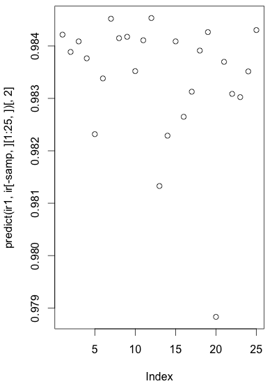
Another way to see this is drawing a plot:
> plot(predict(ir1, ir[-samp,][1:25,])[,2])
where ir[-samp,] is testing data, ir[-samp,][1:25,] is testing data for “Setosa”, and ir[-samp,][1:25,][2,] is output value from neural net for classifying data to “Setosa”.
As we classify those data into “Setosa” only if those values are larger than the values in other columns, we should see large values in this plot.
References)
1. R documentation, “Fit Neural Network”. http://stat.ethz.ch/R-manual/R-devel/library/nnet/html/nnet.html
2. 구자용, 박헌진, 최대우, 김성수, “데이터 마이닝”, Knou Press.
