Robust Regression – Passion is like genius; a miracle.

Classical linear model minimizes $\sum{r_i^2}$ where $r_i$ is residual and called LS(Least Squares) or Sum of Least Squares. But it is not robust against outlier. Thus we need roboust regression methods.

Least Absolute Deviation
Seek to minimize $\sum{|y_i-f(x_i)|}$ . This method has breakdown point zero meaning that even a small number of outliers can damage the goodness of the model. (See Peter J. Rousseeuw’s paper for the discussion of breakdown point here and below.)

M-Estimation
M-Estimation (or M-Estimator) minimizes $\sum{\rho(r_i)}$ . So, in case of LS, $\rho(r_i)=r_i^2$ . Thus, as $r_i$ grows, $\rho(r_i)$ rapidly gets larger. Instead, in Huber’s m-estimation, if $r_i$ is too large, we use linear function so that $\rho$ doesn’t get too big. See Robust Regression by John Fox for details (esp., see the graph of $\rho$ ). However, this method has break down point zero, i.e., is not better than LS in terms of finding robust regression.

Least Median of Squares Regression(LMS)
LMS by Peter J. Rousseeuw miminizes $median(r_1^2, r_2^2, \cdots, r_n^2)$ . Its breakdown point is 50% (which is, according to the paper, is the maximum, as more than 50% contamination of data implies that we can not distinguish good model from the bad one).

Least Trimmed Squares(LTS)
LTS minimizes $\sum_{i}^{k}{r_{(i)}^2}$ when $r_{(i)}$ is sorted as $r_{1}^2 \le r_{2}^2 \le r_{3}^2 \le \cdots \le r_{n}^2$ where $k$ is the number of smallest residuals we pick.

Below is an R example. First, assume that the true function is y = 3x + 1.

> f = function(x) { 3 * x + 1 + rnorm(1) }
> x = 1:20
> d = data.frame(x=x, y=f(x))
> d
    x        y
1   1  4.05855
2   2  7.05855
3   3 10.05855
4   4 13.05855
5   5 16.05855
6   6 19.05855
7   7 22.05855
8   8 25.05855
9   9 28.05855
10 10 31.05855
11 11 34.05855
12 12 37.05855
13 13 40.05855
14 14 43.05855
15 15 46.05855
16 16 49.05855
17 17 52.05855
18 18 55.05855
19 19 58.05855
20 20 61.05855
>

Add some outliers.

> d[18,2]=100
> d[19,2]=200
> d[20,2]=150
> d
    x         y
1   1   4.05855
2   2   7.05855
3   3  10.05855
4   4  13.05855
5   5  16.05855
6   6  19.05855
7   7  22.05855
8   8  25.05855
9   9  28.05855
10 10  31.05855
11 11  34.05855
12 12  37.05855
13 13  40.05855
14 14  43.05855
15 15  46.05855
16 16  49.05855
17 17  52.05855
18 18 100.00000
19 19 200.00000
20 20 150.00000

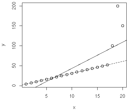
If we plot LMS:

> plot(d)
> abline(lm(y~x, d))
# method lqs is the same with method lms except that it minimizes median considering the number of parameters, thus it's theoretically better according to this book: 허명회, R을 이용한 탐색적 자료분석, 자유아카데미.
> abline(lqs(y~x, method="lqs", d), lty=2)

In the image, dotted line is LMS while solid one is LS.

LTS can be done as:

> plot(d)
> abline(lm(y~x, d))
> abline(lqs(y~x, method="lts", d), lty=3)

This results in the similar plot, so the graph is omitted here.

Now, let’s see if we can find outliers:

> install.packages("car")
> library(car)
> outlierTest(lm(y~x, d), cutoff=Inf, n.max=Inf)
      rstudent unadjusted p-value Bonferonni p
19  5.49881882         3.9131e-05   0.00078263
20  1.49960960         1.5206e-01           NA
17 -1.28017094         2.1768e-01           NA
16 -1.13386920         2.7259e-01           NA
15 -0.99606149         3.3319e-01           NA
14 -0.86502411         3.9907e-01           NA
13 -0.73934044         4.6979e-01           NA
1   0.70856032         4.8820e-01           NA
12 -0.61781396         5.4489e-01           NA
2   0.57102596         5.7545e-01           NA
11 -0.49940495         6.2390e-01           NA
3   0.44052971         6.6510e-01           NA
10 -0.38318240         7.0633e-01           NA
4   0.31548047         7.5624e-01           NA
9  -0.26828556         7.9171e-01           NA
5   0.19456627         8.4804e-01           NA
8  -0.15389138         8.7951e-01           NA
18  0.14042627         8.8997e-01           NA
6   0.07667122         9.3978e-01           NA
7  -0.03918468         9.6920e-01           NA
>

Item 19 and 20 looks suspicious, but outlierTest reports 19 only.

> outlierTest(lm(y~x, d))
   rstudent unadjusted p-value Bonferonni p
19 5.498819         3.9131e-05   0.00078263