> a = aov(iris$Petal.Width ~ iris$Species)
> a
Call:
   aov(formula = iris$Petal.Width ~ iris$Species)

Terms:
                iris$Species Residuals
Sum of Squares      80.41333   6.15660
Deg. of Freedom            2       147

Residual standard error: 0.20465
Estimated effects may be unbalanced

Look. You should call summary on the ret. val of aov to get the following statistics.

> summary(a) 
              Df Sum Sq Mean Sq F value    Pr(>F)   
iris$Species   2 80.413  40.207  960.01 < 2.2e-16 ***
Residuals    147  6.157   0.042                     
—
Signif. codes:  0 ‘***’ 0.001 ‘**’ 0.01 ‘*’ 0.05 ‘.’ 0.1 ‘ ’ 1

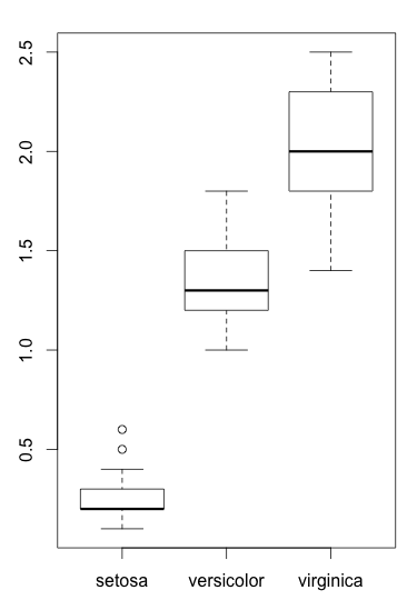
Because P value is very small, H0 is rejected; Petal.Width is different depending on Species.

We can draw a boxplot to visualize this:

Some texts[1] explain that F statistics in ANOVA is (between class variance) / (within class variance) while others say F is (treatment) / (random error), but they basically evaluate the same thing.
ANOVA assumes a couple of things.
a) variance should be the same across classes.
b) error should be independent, and gaussian.
c) data from each class is independent.

In the above, I didn’t do much to show that the assumption holds, but one can run

plot(a)

to get some graphs like ‘residual vs fitted’, ‘qq plot’, etc.

References)
1. http://homepages.inf.ed.ac.uk/rbf/CVonline/LOCAL_COPIES/SHUTLER2/node1.html